

Wins Above Replacement - Part 1: RAPM
Wins Above Replacement - Part 1: RAPM
Meant to write this long ago

This series is meant as an explainer for my WAR model. I intentionally try to keep it light on technical explanations. For people wanting a more details on both WAR models in general and RAPM, I recommend reading the respective parts of the Evolving Hockey References Page, they did an excellent job collecting citations and sources.
Wins Above Replacement, WAR for short, is metric used to quantify a player’s value. It attempts to frame this value in a unit (wins1) people are familiar with and uses a baseline of replaceable players. Wins Above Average would be an almost identical metric to calculate but comparing someone to league average ignores the fact that, for the most part, acquiring a league average player is usually associated with not insignificant costs. The concept of a replacement level player is used to compare to a level of performance which is, in theory at least, easy and cheap to acquire. Be it a player from your team’s academy or on the open market. But more on this later when we’re talking about replacement level players in more detail.
What do we want to measure?
In general we can outline two different goals for our player value metrics:
Accurately describe the value of past performances of a player
Accurately describe a player’s current level of performance
Both these goals are occasionally in conflict. If I just want to talk about the excess value a player has provided me, I would place a lot of value on the actual goals scored. An example:
A player scores 20 goals and has a shooting percentage of 20%+, but his shots only amounted to about 12 expected goals. If we’re looking at this season in isolation, I would have to say: Great, tons of goals, helped the team immensely, provided a lot of value.
But if I am now asked about the quality of this player, I would have to take the high shooting percentage and the large difference between goals and expected goals into account. It seems unlikely that he will be able to repeat this performance, he probably isn’t a "real” 20 goal scorer.
The goal of my WAR model is somewhere in between these two. Obviously I want to provide a metric that can do a good job at judging the most impactful performances. But on the other hand I do not want to credit players for non-repeatable performances and pretend that this is the actual level of play they’re capable of long-term. I wanted to build a model that can provide reasonable answers to both “Who had the best season?” and “Who is the best player?”. Sometimes (for example when looking at Connor McDavid’s recent performances), those answers overlap but they don’t always.
With this in mind we’ll start building our WAR model, starting with the core of the metric: Estimating the on-ice impact on Expected Goals.
My explanation will focus on Even Strength play, but this method is used in a nearly identical way to estimate Powerplay and Penalty Kill impacts.
Why not just use CF%?
What are the typical arguments against using statistics like xGF% (Expected Goals For Percentage) and CF% (Corsi For Percentage)?
Well, it’s ignoring the opposition. ____ is always out there against the opponent’s top players
Well, it’s ignoring context. ____ is out there taking all the defensive zone faceoffs
Well, ____ always gets to play with ________. I’d have good stats playing with him too.
And these complaints aren’t unreasonable. None of them are actually considered in the standard xGF% and CF% metrics (like the ones on 5plusspieldauer.de for example). Even relative to team metrics don’t do much to help this either, they merely account for the strength of the team when the player is not on the ice.
A fictional example: Elias Pettersson suddenly has the urge to play in my beer league hockey team but he really only wants to play with me. So whenever I’m on the ice, so is Elias Pettersson. If I now start tracking the xG ratios of our players during our games, it’ll very quickly look like I’m doing massively better than the rest of my team. Exactly as good as Elias Pettersson, in fact. If these metrics are all that’s at your disposal, you have no way of knowing whether it’s me or EP doing the heavy lifting. Even though it’d be obvious from a few seconds worth of tape.
Obviously this example is extreme, but it illustrates the downsides of the commonly used metrics. The same logic I applied for a teammate obviously also applies for opponents.2 But what to do? How can we isolate the individual impact of a player from the impacts of his teammates and opponents?
Regularised Adjusted Plus Minus
CF% and xGF% are simply the share of shots/expected goals of his team while a given player is on the ice, how do we include information on the other players on the ice in there?
(Very) roughly: We just throw everything into a big regression. Which is to say we look at every shift for every player and look who else was on the ice with them, how many shots (or xG) happened on either side and how long it lasted until someone goes for a change or there’s a break in the play. This is then used to estimate the impact of each players. For only a few shifts and two players, this is comparatively simple:
Shift 1: A + B on the ice, 40s, 2 shots
Shift 2: Just B on the ice, 40s, 0 shots
Shift 3: Just A on the ice, 40s, 2 shots
Seems like whenever Player A is on the ice, two shots happen and whenever he’s not, no shots happen. So we can roughly estimate his impact to be 2 shots (per 40 seconds of time on ice). We do this for every player in our league. For example, in the SHL last season that amounted to about 190.000 sequences (remember, sequences uninterrupted by faceoffs or player changes).
For each sequence, we calculate the length in seconds (shift_length) and the sum of expected goals (xgf) for both sides:
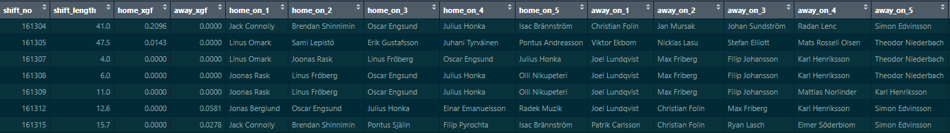
In addition to this we add some more variables. For examples the type of sequence (does it start on the fly or with a faceoff, if it starts with a faceoff, where did that take place and who won it, the strength state, etc.).
Each sequence appears twice in our regression. Obviously if Leksand starts the game by putting up 0 xG in 35 seconds and Luleå put up 0.2 xG we need to credit all the Leksand players with 0 xG offensively and -0.2 xG defensively and all the Luleå players with 0.2 xG offensively and 0 xG defensively, since we’re interested in splitting up the overall impact into offensive and defensive components.
Now we let R loose on this dataset. By using a ridge regression (this paper by Brian MacDonald was very instructive) we can estimate the impacts of all our variables.
RAPM
The results from this regression look roughly like this:
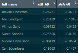
The xG For Impact is the net impact of a player relative to league average on the amount of expected goals that occur for his team whenever he is on the ice (per 60 minutes of play), adjusted for factors like teammates, opponents and other circumstances (like faceoffs/on the fly changes, etc.). Similarly, the xG Against impact is the impact of the player on the opponent’s xG when he is on the ice.
This means that if we put Carl Söderberg out there with 9 completely average SHL players for 60 minutes, we’d expect his team to generate +0.19 xG more than SHL average and allow 0.14 xG less3.
This is what we call RAPM. Regularised Adjusted Plus-Minus4. Plus-Minus simply because you can add up the offensive and defensive impact to get the total impact (for Söderberg +0.19 offensive impact and -0.14 defensive impact, totalling up to + 0.33 xG difference per 60 mins).
The More You Know
Obviously the approach I’ve outlined so far would start every player off on the same level, with the regression knowing nothing about them. But this isn’t necessarily the best approach, since there are players for which we have significant previous information. Would it for example be smart to use the same baseline next season for a player like Carl Söderberg as we’d use for a random prospect coming into the SHL? I don’t think so.5
Therefore we bias our model by informing it about the players in the league for which we have historical data. Good players get a bonus, bad players get a malus, giving our regression some preconceptions about the players we know from previous seasons.
This mainly impacts the extremes, the good and bad players get somewhat larger impacts, especially on offense:
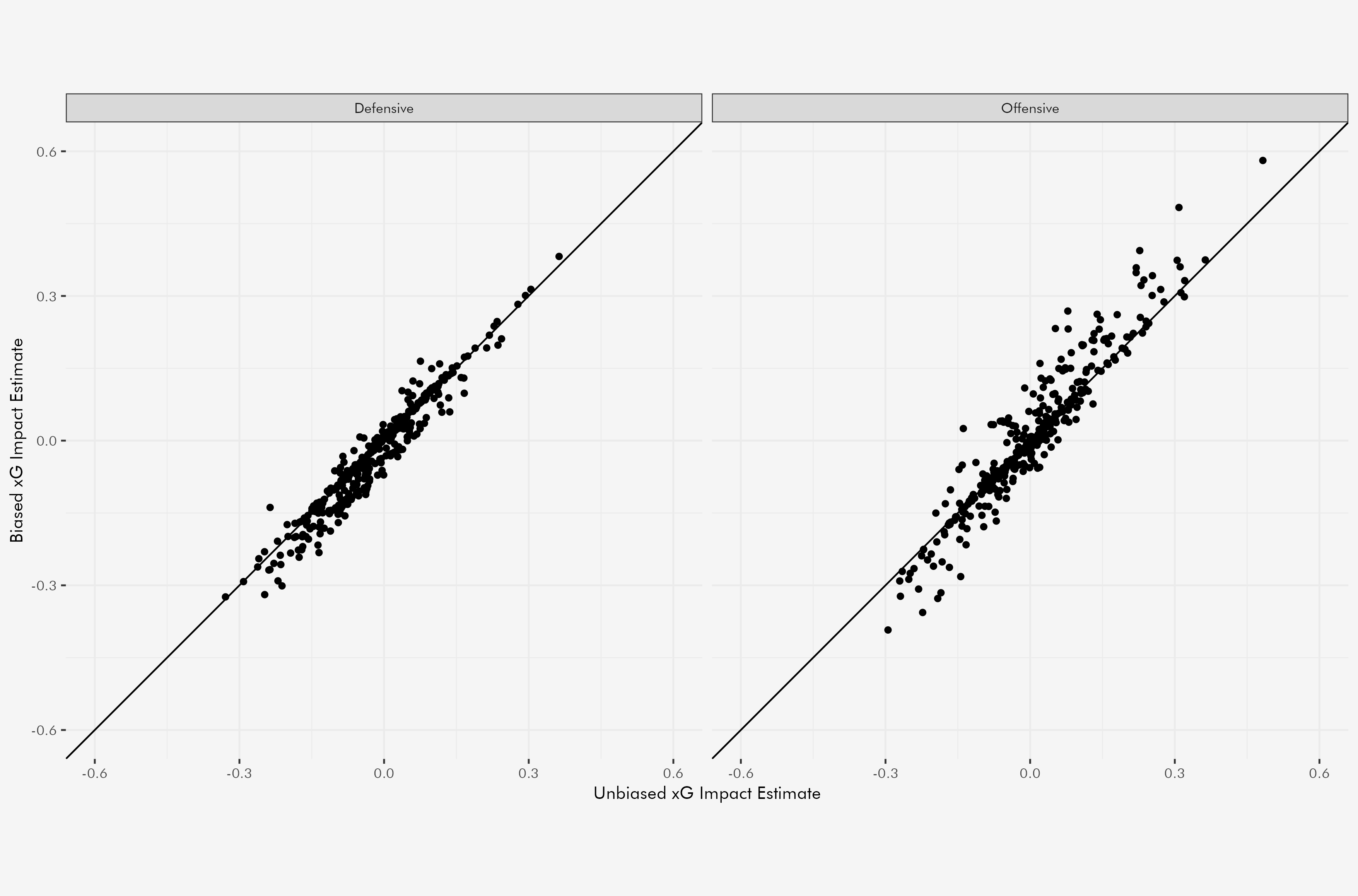
Most players are very close to the diagonal (on which the biased and unbiased impact estimates are identical). From my (admittedly subjective) perspective, the gain achieved by using information from previous seasons outweighs the loss in agility (the “biased” regression has some more inertia when confronted with large changes in performance, players experiencing large changes in performance quality will take longer to fully see these changes reflected in the model outputs).
With RAPM, we can now estimate both the offensive and defensive on ice xG impact of a player. This is by far the most important component of my WAR model. The next post will deal with the additional components (Penalties, Shot Quality, Boxscore Plus Minus) that make my version of Wins Above Replacement.
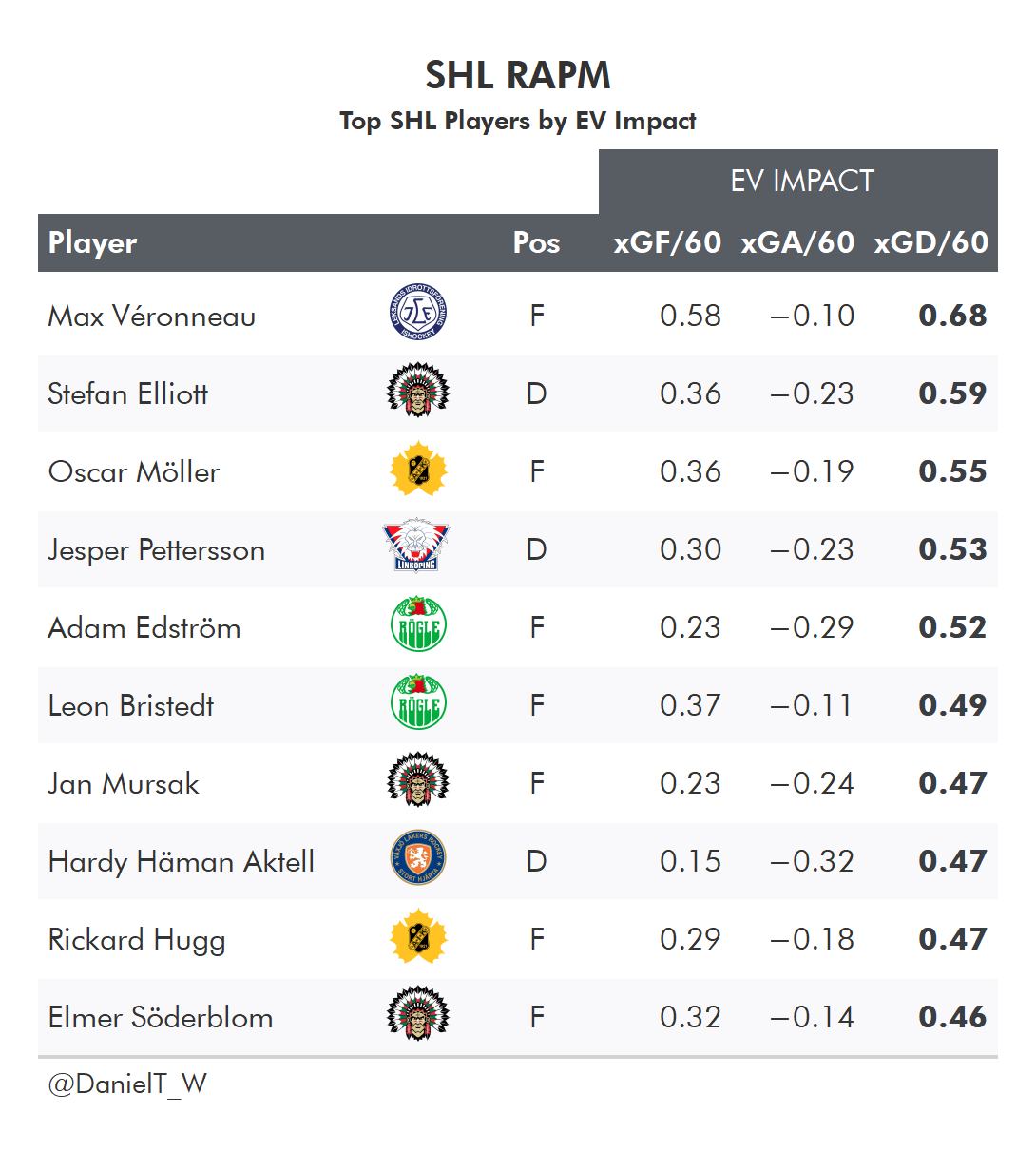
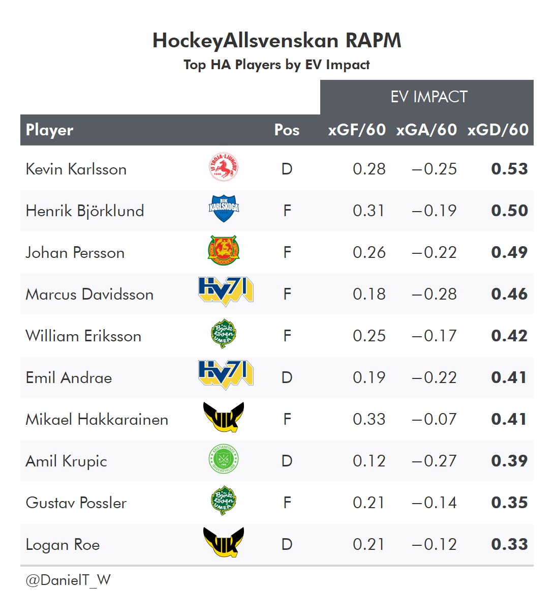
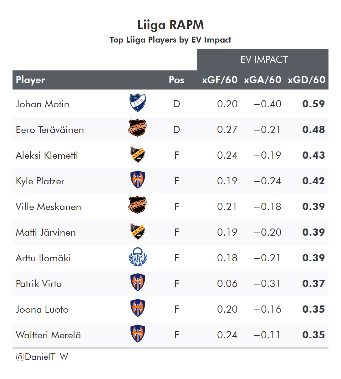
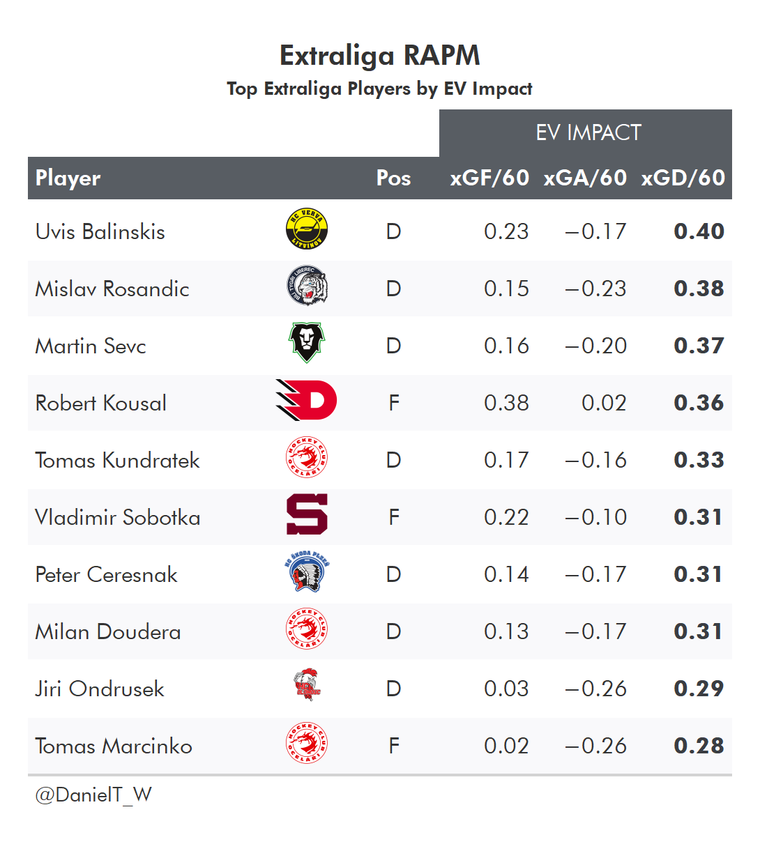
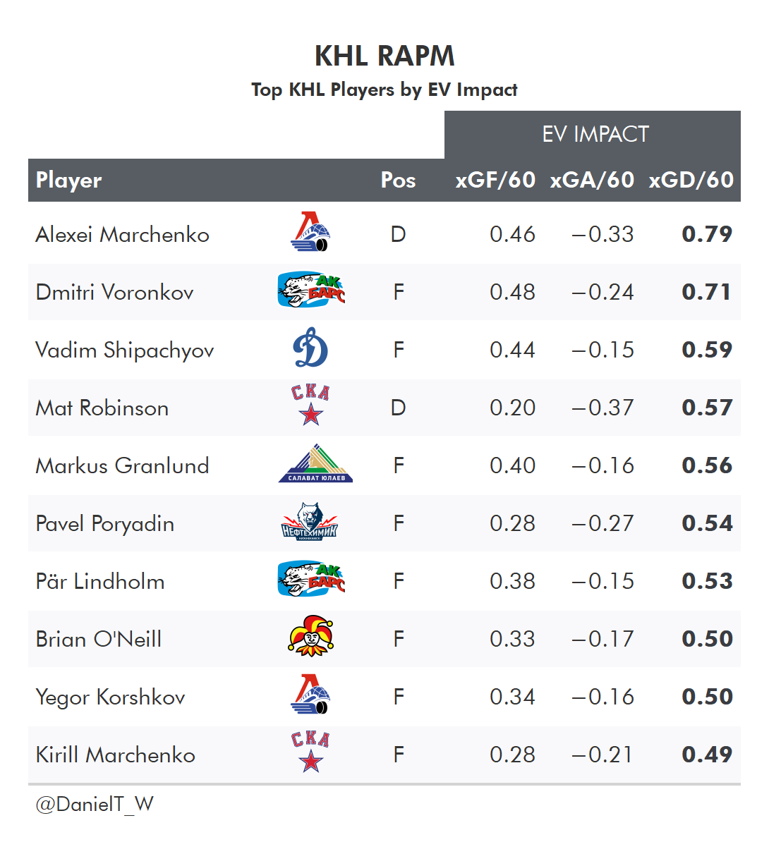
And as a reward for sticking through all these rambling explanations, let’s take a look at the top players by RAPM impacts in 2021/22 for a few leagues:

or Goals (GAR - Goals Above Replacement) or points in the standings (SPAR - Standings Points Above Replacement)
although it is much harder to manage who you’re playing against than who you’re playing with
Keep in mind that with defensive values, lower values are better than higher values since it is about preventing chances. Söderberg therefore allows the opponent 0.14 xG fewer per 60 mins, his impact is +0.14.
“Regularized” here being a mathematical term. For anyone interested in learning more: https://en.wikipedia.org/wiki/Regularization_(mathematics)
There is a debate to be had here, the folks at Evolving Hockey for example do not use priors in their model and prefer to focus on a player’s performance within a single season.